
Simpson's Paradox การรักษานิ่วในไต Stratified Analysis
Simpson's Paradox การรักษานิ่วในไต Stratified Analysis ด้วยโปรแกรม Openepi และ STATA
Simpson's Paradox การรักษานิ่วในไต Stratified Analysis
http://en.wikipedia.org/wiki/Simpson%27s_paradox
http://www.ncbi.nlm.nih.gov/pmc/articles/PMC1339981/?tool=pmcentrez
http://www.ncbi.nlm.nih.gov/pmc/articles/PMC1339981/pdf/bmjcred00227-0031.pdf
http://en.wikipedia.org/wiki/Simpson%27s_paradox
This is another real-life example from a medical study[12] comparing the success rates of two treatments for kidney stones.[13]
http://www.ncbi.nlm.nih.gov/pmc/articles/PMC1339981/pdf/bmjcred00227-0031.pdf
The table shows the success rates and numbers of treatments for treatments involving both small and large kidney stones, where Treatment A includes all open procedures and Treatment B is percutaneous nephrolithotomy:
| Treatment A | Treatment B | |
|---|---|---|
| Small Stones |
Group 1 93% (81/87) |
Group 2 87% (234/270) |
| Large Stones |
Group 3 73% (192/263) |
Group 4 69% (55/80) |
| Both | 78% (273/350) | 83% (289/350) |
การรักษานิ่วในไตวิธี A หรือ B วิธีใหนดีกว่ากัน ?
วิธี A ผ่าตัดนิ่วตามวิธีมาตรฐาน (Open Surgery)
วิธี B วิธีใช้เครื่องสลายนิ่ว (ESWL)
วิธี A ผ่าตัดนิ่วตามวิธีมาตรฐาน (Open Surgery)
วิธี B วิธีใช้เครื่องสลายนิ่ว (ESWL)
Small stones (+) (-)
A 81 6 87
B 234 36 270
B 234 36 270
Large stones (+) (-)
A 192 71 263
B 55 25 80
B 55 25 80
A = 93% (81/87) > B = 87% (234/270)
A = 73% (192/263) > B = 69% (55/80)
A = 78% (273/350) < B = 83% (289/350)
วิธี A ดีกว่าถ้าก้อนนิ่วมีขนาดเล็ก A = 93%
วิธี A ดีกว่าถ้าก้อนนิ่วมีขนาดใหญ่ A = 73%
วิธี B ดีกว่าถ้ารวมกันทั้งนิ่วก้อนเล็กและนิ่วก้อนใหญ่ B = 83%
การรวมกันแบบ Crude บางครั้งจะไม่ถูกต้อง เพราะมี Confounding หรือ Effect Modfication หรือมีทั้งสองอย่าง
Crude (+) (-)
A 273 77 350
B 289 81 350
B 289 81 350
1) นิ่วก้อนเล็กวิธี A ดีกว่า
2) นิ่วก้อนใหญ่วิธี A ดีกว่า
3) ถ้ารวมกันทั้งนิ่วก้อนเล็กและใหญ่ วิธี B ดีกว่า ?
4) ใช้ M-H Adjusted Risk Ratio หรือ M-H Adjusted Odds Ratio
ซึ่ง Lurking Variable ก็คือ Confounder; M-H Adjusted Stratified Analysis จะแสดงให้เห็นว่า "การรวมกันแบบ Crude มี Confounder หรือไม่? มี Effect Modification หรือไม่?" เป็นการตรวจสอบในขั้นตอนการวิเคราะห๋ ถ้าเป็นไปได้ ในขั้นตอน Study Design ควรออกแบบ Clinical Trial ให้เป็น Randomized เพื่อให้นิ่วก้อนเล็กและก้อนใหญ่ได้รับการรักษา ด้วย วิธี A และฺวิธี B โดยมีอัตราส่วนเท่า ๆ กัน ซึ่งใน Study นี้ไม่ได้เป็นเช่นนั้น
นิ่วก้อนเล็กใช้วิธี A : B = 87 : 270
นิ่วก้อนใหญ่ใช้วิธี A : B = 263 : 80
คือนิ่วก้อนเล็กจะใช้วิธีเครื่องสลายนิ่วคือวิธี B (ESWL) ก่อน ถ้าไม่ได้ผลสามารถจะใช้ วิธี A (Open Surgery) ได้ในภายหลัง นิ่วก้อนใหญ่คาดว่าคงจะใช้วิธี B ไม่ผลดีนัก จึงใช้วิธี A มากกว่า
The paradoxical conclusion is that treatment A is more effective when used on small stones, and also when used on large stones, yet treatment B is more effective when considering both sizes at the same time.
เมื่อแยกกัน นิ่วก้อนเล็กวิธี A ดีกว่า, นิ่วก้อนใหญ่วิธี A ดีกว่า
เมื่อนำมารวมกัน นิ่วก้อนเล็กรวมกับนิ่วก้อนใหญ่วิธี B ดีกว่า
จะตอบว่า วิธี A ดีกว่า ? หรือ วิธี B ดีกว่า ?
Mantel Haenszel Adjusted Analysis สามารถตรวจสอบว่าการรวมกันแบบ Crude มี Confounder และหรือ มี Effect Modification อยู่ด้วยหรือไม่ ? โดยการแยกวิเคราะห์ทีละกลุ่ม โดยวิธี Stratified analysis ตามตัวอย่างตอนท้ายของบทความนี้โดยโปรแกรม Openepi และ STATA
Mantel Haenszel Adjusted Analysis สามารถตรวจสอบว่าการรวมกันแบบ Crude มี Confounder และหรือ มี Effect Modification อยู่ด้วยหรือไม่ ? โดยการแยกวิเคราะห์ทีละกลุ่ม โดยวิธี Stratified analysis ตามตัวอย่างตอนท้ายของบทความนี้โดยโปรแกรม Openepi และ STATA
ตัวเลขในวงเล็บคือสัดส่วน (Proportion)
การรักษาได้สำเร็จ (Success) หารด้วยจำนวนทั้งหมด (Total)
การรักษาได้สำเร็จ (Success) หารด้วยจำนวนทั้งหมด (Total)
A B
Small stones 93% (81/87) 87% (234/270)
Large stones 73% (192/263) 69% (55/80)
Small stones (+) (-)
A 81 6
B 234 36
B 234 36
Large stones (+) (-)
A 192 71
B 55 25
B 55 25
Crude (+) (-)
A 273 77 350
B 289 61 350
B 289 61 350
Kidney stone treatment
The paradoxical conclusion is that treatment A is more effective when used on small stones, and also when used on large stones, yet treatment B is more effective when considering both sizes at the same time. In this example the "lurking" variable (or confounding variable) of the stone size was not previously known to be important until its effects were included.
(Add Stratum) Stratum ที่ 2
192 71
55 25


Breslow-Day test for interaction of OR, p greater than 0.05 does not suggest interaction. Adjusted OR can be used. Editor's choice = Mid-P Exact.
OpenEpi จัดให้ Exp(+) Exp (-) ไว้ด้านซ้าย, Cases และ Control อยู่ด้านบนของ 2x2 table
โปรแกรมสถิติ STATA จัดให้ Exposed และ Unexposed ไว้ด้านบน, Cases และ Controls อยู่ด้านซ้าย ของ 2x2 table
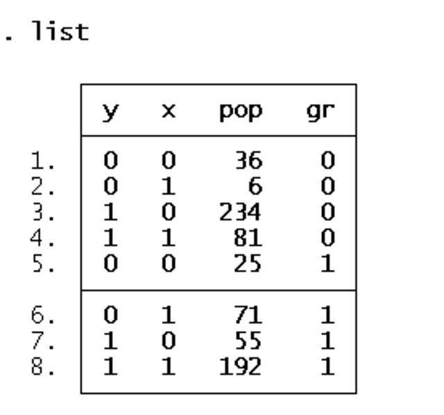
y คือ row (0=Controls, 1=Cases)

Which treatment is considered better is determined by an inequality between two ratios (successes/total). The reversal of the inequality between the ratios, which creates Simpson's paradox, happens because two effects occur together:
- The sizes of the groups, which are combined when the lurking variable is ignored, are very different. Doctors tend to give the severe cases (large stones) the better treatment (A), and the milder cases (small stones) the inferior treatment (B). Therefore, the totals are dominated by groups three and two, and not by the two much smaller groups one and four.
- The lurking variable has a large effect on the ratios, i.e. the success rate is more strongly influenced by the severity of the case than by the choice of treatment. Therefore, the group of patients with large stones using treatment A (group three) does worse than the group with small stones, even if the latter used the inferior treatment B (group two).
M-H Adjusted Stratified Analysis
จะแสดงให้เห็นว่าการรวมกันแบบ Crude มี Confounder หรือไม่ มี Effect Modification หรือไม่
ท่านผู้อ่าน อาจทดลอง M-H Stratified Analysis ที่ www.openepi.com ในหมวด Counts เลือก 2x2 table
จะแสดงให้เห็นว่าการรวมกันแบบ Crude มี Confounder หรือไม่ มี Effect Modification หรือไม่
ท่านผู้อ่าน อาจทดลอง M-H Stratified Analysis ที่ www.openepi.com ในหมวด Counts เลือก 2x2 table
Stratum ที่ 1
81 6
234 36
234 36
(Add Stratum) Stratum ที่ 2
192 71
55 25
1) Stratum 1 OR = 2.07 95%CI 0.84 to 5.11
2) Stratum 2 OR = 1.22 95%CI 0.71 to 2.12
3) Crude OR = 0.74 95%CI 0.51 to 0.10
4) M-H Adj. OR = 1.44 95%CI 0.91 to 2.28
3) Crude OR = 0.74 95%CI 0.51 to 0.10
4) M-H Adj. OR = 1.44 95%CI 0.91 to 2.28
Breslow-Day test for interaction of OR, p greater than 0.05 does not suggest interaction. Adjusted OR can be used. Editor's choice = Mid-P Exact.
OpenEpi จัดให้ Exp(+) Exp (-) ไว้ด้านซ้าย, Cases และ Control อยู่ด้านบนของ 2x2 table
(+) (-)
Exp (+) a, b
Exp (-) c, d
Exp (+) a, b
Exp (-) c, d
(ตั้งค่า Openepi ที่เป็น Epiinfo Layout ให้เป็นแบบ Kleinbaum; Breslow/Day ได้)
โปรแกรมสถิติ STATA จัดให้ Exposed และ Unexposed ไว้ด้านบน, Cases และ Controls อยู่ด้านซ้าย ของ 2x2 table
y คือ row (0=Controls, 1=Cases)
x คือ col (0=Unexposed, 1=Exposed)
pop คือจำนวน เพื่อใช้เป็น freq weight [fw=pop]
gr คือ group 0, 1
gr คือ group 0, 1
คำสั่ง STATA เพื่อหาค่า Odds Ratio ของ gr0, gr1 และ Crude ซึ่งจะแสดงค่า a, b c, d ใน 2x2 table
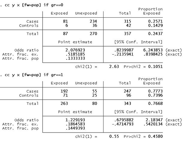
.cc y x [fw=pop] if gr==0
.cc y x [fw=pop] if gr==1
.cc y x [fw=pop] if gr==0
.cc y x [fw=pop] if gr==1
.cc y x [fw=pop]
.cc y x [fw=pop], by(gr)
Mentel-Haenszel Adjusted ซึ่งจะแสดงค่า OR ของแต่ละ group, Crude และ M-H Adjusted OR (แต่ M-H จะไม่ได้แสดง 2x2 table)
.cc y x [fw=pop], by(gr)
Mentel-Haenszel Adjusted ซึ่งจะแสดงค่า OR ของแต่ละ group, Crude และ M-H Adjusted OR (แต่ M-H จะไม่ได้แสดง 2x2 table)
1) gr_0 วิธี A ดีกว่า OR = 2.07 95%CI = 0.82, 6.24
แต่ว่า gr_0, gr_1, Crude และ M-H Adjusted ทั้ง 4 ข้อ 95% Conf. Interval ของ Odds Ratio มีค่า 1 รวมอยู่ด้วย Odds Ratio จึงมีโอกาสเท่ากับ 1 ได้
2) gr_1 วิธี A ดีกว่า OR = 1.22 95%CI = 0.67, 2.18
3) Crude วิธี B ดีกว่า OR = 0.74 95%CI = 0.50, 1.10
4) M-H combined วิธี A ดีกว่า OR = 1.44 95%CI = 0.91, 2.28
4) M-H combined วิธี A ดีกว่า OR = 1.44 95%CI = 0.91, 2.28
(1) OR gr_0 = 2.07 OR มากกว่า 1
(2) OR gr_1 = 1.22 OR มากกว่า 1
(2) OR gr_1 = 1.22 OR มากกว่า 1
(3) Crude OR =0.74 OR น้อยกว่า 1 กลับทิศทางกับ (1) และ (2)
(4) ใช้ M-H ปรับแก้ จึงได้ค่า M-H Adjusted OR = 1.44
แต่ว่า gr_0, gr_1, Crude และ M-H Adjusted ทั้ง 4 ข้อ 95% Conf. Interval ของ Odds Ratio มีค่า 1 รวมอยู่ด้วย Odds Ratio จึงมีโอกาสเท่ากับ 1 ได้
หมายเลขบันทึก: 439144เขียนเมื่อ 13 พฤษภาคม 2011 07:24 น. ()แก้ไขเมื่อ 11 ธันวาคม 2012 13:43 น. () สัญญาอนุญาต: ครีเอทีฟคอมมอนส์แบบ แสดงที่มา-ไม่ใช้เพื่อการค้า-อนุญาตแบบเดียวกันจำนวนที่อ่านจำนวนที่อ่าน:
ความเห็น (0)
ไม่มีความเห็น